Stochastics

VIMC modelling groups produce stochastic data for us, which is currently 200 runs of their models varying key parameters, to express uncertainty. These files get uploaded to Box, and the groups are provided with guidance to produce files that we can process easily.

Stoner can process these stochastic files into a standard format to make the files more predictable to work with. For a good compromise between ease-of-use, performance and compression, we have used the Parquet format and the arrow package. This vignette covers how to process the data, how to create a central from a set of stochastics, how to produce some graphs of the stochastics for quick diagnosis, and also how to use the stochastic explorer, a local shiny app for exploring and comparing stochastic datasets.

Creating standard stochastic files

This has superseded stoner_stochastic_process, which will be removed and undocumented soon.

Here, we are mostly likely working with two folders or network shares, one of which contains the stochastics that groups have uploaded, and the other is a destination where we want to write our standardised files. These I’ll call in_path and out_path. The out_path folders I am assuming will be only written to by stoner; paths and filenames will adhere to the following format:-

Within the root of the share we will have the touchstone, without a version. At time of writing, we have 202310gavi and 202409malaria. I am not anticipating having separate stochastics for separate versions of the stochastics at this point.
Within those touchstone folders, we have more folders in the form Disease_Modelling-Group - such as COVID_IC-Ghani or YF_IC-Garske. The groups and diseases set up here copy the historic contents of the Montagu database.
Within each of these folders, we will be writing a file per country per scenario, containing all run_ids, named in the format Modelling-Group_scenario_country.pq - for example, IC-Garske_yf-routine-ia2030_KEN.pq. If we also create a average (central) of the stochastics (see later), that will be called IC-Garske_yf-routine-ia2030_central.pq, containing all the countries, and no run_id.
Finally, in the root of the standardised folder, we’ll keep a file meta.csv to describe in one file the range of stochastic data we have by touchstone, disease, group and scenario, and for each the outcomes and countries provided. This is useful for speeding up the stochastic explorer shiny app, but also may be a useful quick reference of our inventory in general.

Example Usage - One file per scenario

Examples used so far are in the scripts folder in the root of the stoner repo - files such as process_stoch_202310gavi.R. Here is an example of the Yellow Fever standardisation:-

scenarios = c("yf-no-vaccination", "yf-routine-bluesky",
              "yf-routine-campaign-bluesky", "yf-routine-campaign-default",
              "yf-routine-campaign-ia2030", "yf-routine-default",
              "yf-routine-ia2030")

stoner::stone_stochastic_standardise(
  group = "IC-Garske",
  in_path = file.path(base_in_path, "YF-IC-Garske"),
  out_path = file.path(base_out_path, "YF_IC-Garske"),
  scenarios = scenarios,
  files = "burden_results_stochastic_202310gavi-3_:scenario Keith Fraser.csv.xz")

base_in_path and base_out_path are defined elsewhere, and are my drive mappings to the incoming, and destination network shares. We’ll briefly talk about those later.

We provide the group name, the paths to the uploaded files and the destination we want to write files to. Note that the in_path is not managed, and might be arbitrary - here it has dashes instead of underscores; but the out_path, we need to be careful to get right, in the format disease then underscore then the modelling group.

We then provide the vector of scenarios, and because this group follow the guidance very well, they have included the exact scenario in the filenames. We can therefore use the :scenario glob in the files argument, and stoner will handle each of the seven scenarios in the right order.

Example Usage - One file per run

Other groups provide a file per run, which is also fine. Here, we can specify an additional index parameter, usually 1:200, and use the glob :index in the files argument. Here is an example of that - but note for this group, they didn’t quite include the scenarios exactly in the filenames, so we have to explicitly name the files, rather than using the :scenario glob. This is still yellow fever, so using the same scenarios vector as before.

stoner::stone_stochastic_standardise(
  group = "UND-Perkins",
  in_path = file.path(base_in_path, "YF-UND-Perkins"),
  out_path = file.path(base_out_path, "YF_UND-Perkins"),
  scenarios = scenarios,
  files = c("stochastic_burden_est_YF_UND-Perkins_yf-no_vaccination_:index.csv.xz",
            "stochastic_burden_est_YF_UND-Perkins_yf-routine_bluesky_:index.csv.xz",
            "stochastic_burden_est_YF_UND-Perkins_yf-routine_campaign_bluesky_:index.csv.xz",
            "stochastic_burden_est_YF_UND-Perkins_yf-routine_campaign_default_:index.csv.xz",
            "stochastic_burden_est_YF_UND-Perkins_yf-routine_campaign_ia2030_:index.csv.xz",
            "stochastic_burden_est_YF_UND-Perkins_yf-routine_default_:index.csv.xz",
            "stochastic_burden_est_YF_UND-Perkins_yf-routine_ia2030_:index.csv.xz"),
  index = 1:200)

The subtle difference is that the group used underscores instead of dashes in the scenario names. So here, I have to be careful and ensure the order of files matches the order of scenarios manually. After that, the :index glob, and the index argument deal with the fact we have 200 files per scenario.

Example Usage - One file per country

If groups want to supply a file per country, then at present, we need them to do so including the country in their uploads as normal, but number their files using the index method above, rather than having country names or ISO codes in the filename. We could do better if this proves to be a popular method.

Updating the meta-data

Having run stone_stochastic_standardise and made changes to the structure, to enable the stochastic explorer shiny app to use the data (and to keep a useful file up-to-date), we need to run a command to update the metadata.

stoner::stone_stochastic_make_meta(out_path)

which will run for a few seconds, recreating the entire file. The columns are touchstone, disease, group, scenario, countries and outcomes; the first four will be single elements, whereas countries and outcomes will be semi-colon separated lists.

Advanced Usage

You shouldn’t have to worry about these things, but this is just so that you know they are there. We have some historic fixes that have made it possible for us to process some groups’ stochastics with some formatting issues, rather than asking them to resubmit. These fixes are enabled by default; they won’t do anything bad for groups where the fixes are not relevant, and are strictly required for the groups where they are relevant.

The Rubella Fix

An argument rubella_fix, by default TRUE, deals with the fact that rubella groups have traditionally uploaded with different outcome names. Instead of deaths, rubella_deaths_congenital, and instead of cases, rubella_cases_congenital. Some groups additionally supplied the rubella_infections outcome.

The rubella_fix argument causes stoner to omit rubella_infections, and rename the others to deaths and cases respectively, standardising them against the other diseases.

The Missing Run Id fix

One group also is in the habit of sending us one file per run_id, but omitting the run_id field from their uploads. The argument missing_run_id_fix, default TRUE lets Stoner spot this, and specifically if index is 1:200 (ie, we are expecting 200 uploads), it will transplant the index into the file to allow processing to be done normally.

Other Considerations:

Stoner rounds of all the outcomes, (deaths, cases, dalys, yll and cohort_size) to be integer-like, which can create some confusion with small countries with a very small number of cases, but we expect those confusions. Some groups still provide us with 16 decimal places, which creates some problems, and the integer-like rounding is in the guidance.
Note that for some groups with very large files (especially those with 16 decimal places), the processing takes a lot of memory - towards 128Gb. So run these on a large machine or perhaps a cluster node.

More about the paths

If at all possible, you should perform Stoner tasks on a computer within DIDE, connected with a cable. Stochastic processing involves large volumes of data, and ZScaler from outside, or even WiFi from inside may not copy that well with these tasks.

On a DIDE Windows machine, in_path and out_path can be fully-qualified paths to DIDE network shares, which only members of the VIMC team have access to. This is probably the easiest case.

On Linux or Mac, you have to mount the DIDE network shares, providing your DIDE details, and it is up to you what you call your local mountpoints. On linux, they may start with /mnt/ and on Mac /Volume/. Talk to IT, if you need help setting up those mounts.

And lastly, if you’re on a windows machine but for some reason need to work externally, then use ZScaler, map drive letters to the network shares, and pass those in, but as we said, this is not recommended as it’s not particularly stable. If at all possible, use an internal machine to do the heavy data work, and remote desktop into that if you need to be external.

Creating a central estimate

For many groups, their central estimates are the average of their stochastic runs. Historically groups have provided their centrals before their stochastics, as a means of early review and detection of problems. Having standardised a group’s stochastic files, we can then generate an averaged central for a single touchstone, disease, group and scenario, with the following call:-

stone_stochastic_central(base, "202310gavi", "YF", "IC-Garske", 
                         "yf-routine-campaign-ia2030")

base here is the root of the share where our standardised stochastic outputs have been put, and since those were created by stoner, it knows how to build the paths correctly.

The result will be a new file in the form group_scenario_central.pq so in this case IC-Garske_yf-routine-campaign-ia2030_central.pq which matches the other standardised filenames, except for the country; this one central file will contain all countries.

The default averaging function is mean - if we really want the median of the stochastics, then add the argument avg_method = mean to the function call. Note the lack of quotes - we are sending a function, not the name of a function.

Creating stochastic graphs

The stone_stochastuc_graph function can dig out a range of different graphs. If you want to explore the stochastics interactively, then try the shiny app (below) - but for programmatic plotting, read on.

Basic burdens.

With base set to the root of the share where we are putting our standardised outputs, here is an example function call, and the graph that it produces.

stone_stochastic_graph(base, "202310gavi", "YF", "IC-Garske",
                       "KEN", "yf-no-vaccination",
                       "deaths")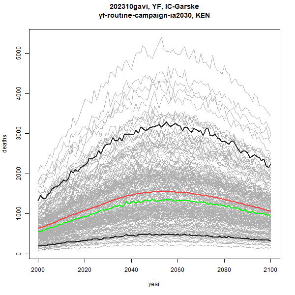

The grey lines are each and every stochastic run. Red is the mean, and green is the median of the stochastics. The thicker black lines are the 5% and 95% quantiles. We can toggle the presence of each of those line types with the optional arguments include_stochastics, include_quantiles, include_mean and include_median, which can be set to FALSE, or left as the default TRUE.

Burden Differences

If we specify two scenarios instead of one, then the plot will be the burden of the first scenario, subtract the burden of the second - i.e., the difference made by applying a scenario. Below is an example - I’ll also add the log = TRUE argument to get a logged y-axis.

stone_stochastic_graph(base, "202310gavi", "YF", "IC-Garske",
                       "KEN", c("yf-no-vaccination", "yf-routine-campaign-ia2030"),
                       "deaths", log = TRUE)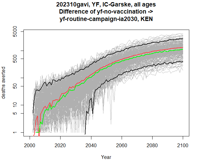

The y-axis now reads “deaths averted” instead of just deaths.

Comparing touchstones

You may have noticed that stone_stochastic_graph when you run it causes a plot to appear, but is actually returning you a list of plots - one so far. If we specify two touchstones, then stoner will instead return us a list of two graphs - assuming that the same disease, group and scenarios are present in both touchstones. The y-axis will be matched between the two, so we can see the pair of graphs for comparison.

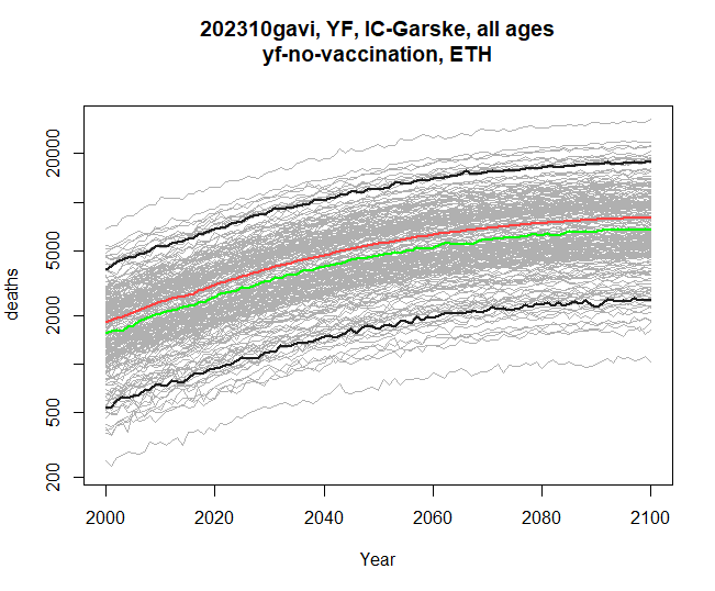
Below is an example returning to just a single scenario, although you can provide two and compare burden differences across two touchstones too. Here I am collecting both resulting graphs, and then plotting them one by one.

res <- stone_stochastic_graph(base, c("202110gavi", "202310gavi"), "YF", "IC-Garske",
                       "ETH", "yf-no-vaccination",
                       "deaths", log = TRUE)
res[[1]]
res[[2]]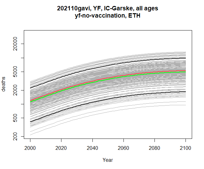

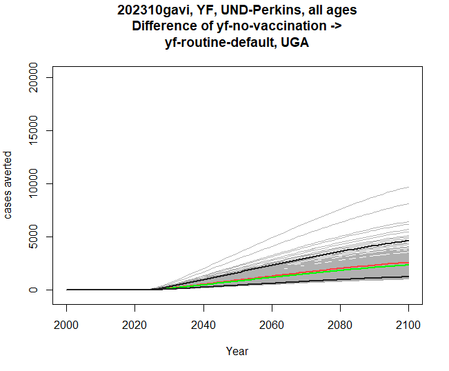
Comparing modelling groups

Similarly, within the same touchstone, we can compare two modelling groups, with either a single scenario, or pair of scenarios. The disease, scenarios and outcomes must be compatible between the two groups. Here’s a comparison of burden difference:

res <- stone_stochastic_graph(base, "202310gavi", "YF", 
                              c("IC-Garske", "UND-Perkins"),
                              "UGA", 
                              c("yf-no-vaccination", "yf-routine-default"),
                              "cases")
res[[1]]
res[[2]]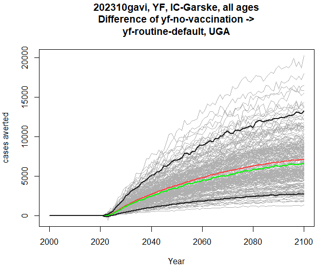

Filtering by age

The stochastic data contains both years and ages. Our plots so far have been using time on the x-axis, and all the ages have been summed together for each calendar year. We can also filter by age before plotting. The example below filters to ages between 0 and 4 inclusive (ie, under 5 year-olds).

res <- stone_stochastic_graph(base, "202310gavi", "YF", "IC-Garske", "UGA",
"yf-no-vaccination", "deaths", filter = 0:4)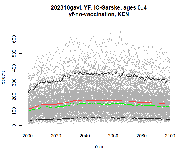

Plotting by birth cohort

The by_cohort parameter lets us subtract age from year before plotting, so we can see burden specific to people who were born in a certain year, rather than the previous plots, which have all treated the x-axis as calendar year.

res <- stone_stochastic_graph(base, "202310gavi", "YF", "IC-Garske", "UGA",
                              "yf-no-vaccination", "deaths", by_cohort = TRUE)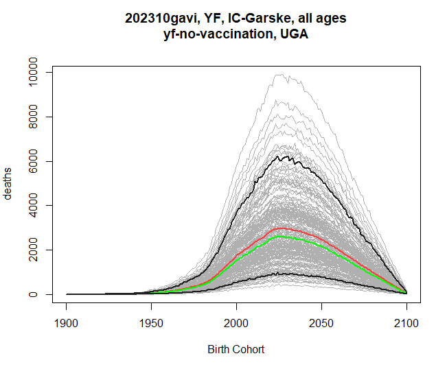

Age on the x-axis

If instead we want to see how burden affects people of different ages throughout the time series, we can set xaxis to age (its default is time).

res <- stone_stochastic_graph(base, "202602yf", "YF", "IC-Gaythorpe", "UGA",
                              "yf-no-vaccination", "deaths", xaxis = "age")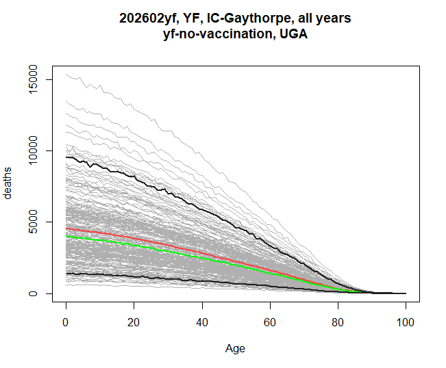

This sums over the entire range of years. If xaxis is age, then the filter argument will let you select which years are to be included. This example shows the burden by age in the years 2040-2050.

res <- stone_stochastic_graph(base, "202602yf", "YF", "IC-Gaythorpe", "UGA",
                              "yf-no-vaccination", "deaths", xaxis = "age",
                              filter = 2040:2050)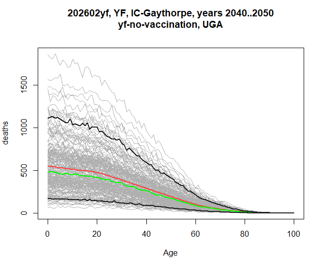

And if we additionally set the by_cohort flag, then we are asking for the burden breakdown by age, for people who were born within the filtered range, rather than selecting a calendar year range.

res <- stone_stochastic_graph(base, "202602yf", "YF", "IC-Gaythorpe", "UGA",
                              "yf-no-vaccination", "deaths", xaxis = "age",
                              filter = 2040:2050, by_cohort = TRUE)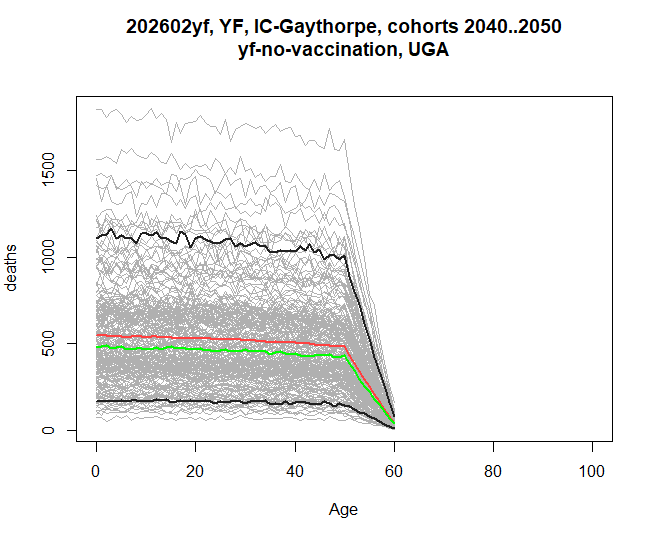

The graph has this shape because the stochastics here only continue until 2100, hence the last 60-year olds will be born in 2040.

Including data from packit.

Lastly, if a central burden estimate has been included in a packit in Montagu’s reporting portal, we can include that on a graph by specifying the id, and the name of the file within that packit. For example, this graph shows both the stochastics from the file share, and the central from a packit, which is drawn in blue.

res <- stone_stochastic_graph(base, "202602yf", "YF", "IC-Gaythorpe", "UGA",
                              "yf-no-vaccination", "deaths", 
                              packit_id = "20260421-090519-e4a90228",
                              packit_file = "burden-estimates-disaggregated.rds")

Visit <https://montagu.vaccineimpact.org/packit/device> and enter code DNLH-NMRL

✔ Waiting for response from server [10.6s]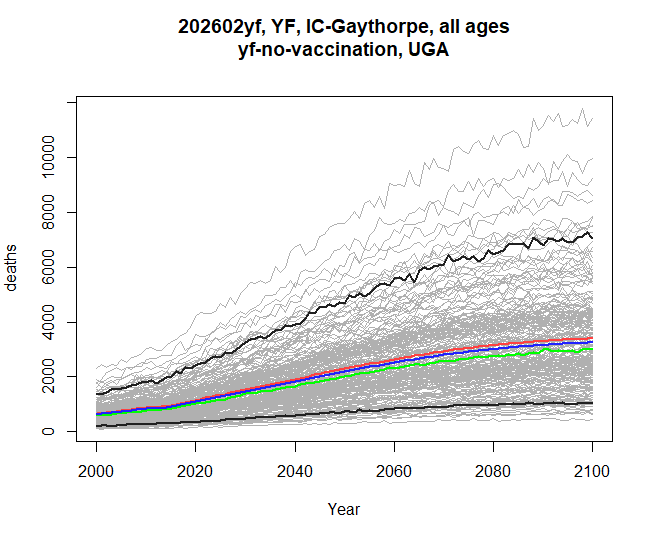

And here’s an example of a burden difference graph, showing how much difference the yf-routine-default scenario makes in both the stochastics, and the central from packit.

res <- stone_stochastic_graph(base, "202602yf", "YF", "IC-Gaythorpe", "UGA",
                               c("yf-no-vaccination", "yf-routine-default"), "deaths", 
                               packit_id = "20260421-090519-e4a90228",
                               packit_file = "burden-estimates-disaggregated.rds")

Visit <https://montagu.vaccineimpact.org/packit/device> and enter code MBWV-NBBC
✔ Waiting for response from server [10.9s]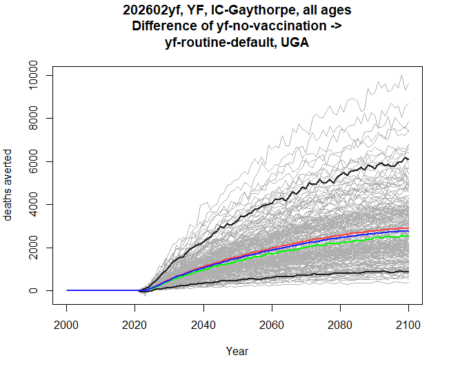

## The stochastic explorer shiny app

All of the graphs above (except currently the packit graphs) can be visualised interactively using a shiny app that is part of stoner. We call it providing the path to the root of the standardised stochastic data, where the meta.csv file should also be found.

stoner::stochastic_explorer(path)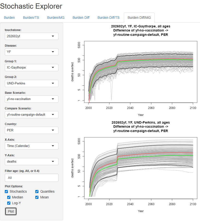

The features in the GUI closely map onto the parameters for stochastic_graph in the following ways:

The tabs along the top let you choose a single graph, a comparison by touchstone, or a comparison by modelling group, firstly for simply burdens, and secondly for differences between scenarios. Different tabs therefore cause different components in the sidebar to be available.
One or two touchstones, groups, or scenarios will be available depending on the tab.
Whether the x-axis is time or age, and whether by cohort, are all selected in the x-axis dropdown.
The filter text, whether for time or for age, is a comma-separated list of numbers or dash-separated ranges. So in a contrived example, 0-5,50,95-100 would select the very young, very old, and exactly 50-year olds.

Stochastics

Wes Hinsley

2026-06-23

Stochastics

Creating standard stochastic files

Example Usage - One file per scenario

Example Usage - One file per run

Example Usage - One file per country

Updating the meta-data

Advanced Usage

The Rubella Fix

The Missing Run Id fix

Other Considerations:

More about the paths

Creating a central estimate

Creating stochastic graphs

Basic burdens.

Burden Differences

Comparing touchstones

Comparing modelling groups

Filtering by age

Plotting by birth cohort

Age on the x-axis

Including data from packit.